🧠🏷️ Selection of experience for memory by hippocampal sharp wave ripples
The companion notebook will walk you through the steps of trial identity decoding form spiking data!
🔗 Follow the demo code in Colab Notebook here! You will learn how to decode trial identity from population activity using four different methods!
Part 1: How does UMAP work?
UMAP is an algorithm for dimension reduction based on manifold learning techniques and ideas from topological data analysis.
At a very high level, UMAP is comprised of two main steps:
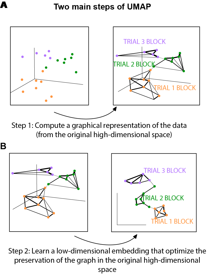
- Step 1: compute a graph representing your data in the high dimensional space (Fig. 1A).
- In some sense in the end we have simply constructed a weighted graph where the weight is an aproxy of the distance between two data points in the high-dimensional space. Fig. 1 was designed to help us gain an intuitive understanding of this. As illustrated in Fig.1A, if two points are close to each other, the weight connecting the two are bigger, which corresponds to a thicker edge connecting the dots in Fig.1A.
- If you want to dig deeper into the theory, you can read more about the topological data analysis and simplicial complex theory behind this step here, but at the implementational level, the Nearest-Neighbor-Descent algorithm of Dong et al. was implemented.
- Step 2: learn a low-dimensional embedding that preserves the structure of the graph as much as possible (Fig.1B).
- This step is essentially solving an optimization problem. Stochastic gradient descent was applied for the optimization process. The negative sampling trick (as used by word2vec) was used to speed up the computation.
I recommend watching this talk if you are looking for an in-depth overview of UMAP. If you are looking for the mathematical description, please see the UMAP paper.
Part 2: Supervised dimensionality reduction
In order to better visualize the trial-by-trial representation drift and check if the progression of population representation drift aligns with the order of the events, we took advantage of the supervised dimensionality reduction feature of the UMAP.
For unsupervised dimensionality reduction,the only input to the UMAP algorithm is the spiking data. For supervised dimensionality reduction, we also pass the class membership (in this case trial identity) as input. We can simply pass the UMAP model the trial label with the following code when fitting , and UMAP will make use of it to perform supervised dimension reduction! It is very easy!
embedding = umap.UMAP().fit_transform(data, y=trial_label)
How does UMAP make use of the trial label information under the hood? When optimizing the low-dimensional embedding, UMAP will pack the data with the same class label closer to each other while push the data with different label far away from each other.
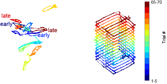
As described in the first demo, we record from many hundreds of neurons simultaneously in the dorsal CA1 region of the hippocampus while the animal perform the figure-8 maze task. We plotted the result of supervised dimensionality reduction with UMAP as interactive plots below. We first colored the manifold with linearized position of the mouse (Fig. 2) and then colored it with trial block number (Fig. 3). The left panel is the neural manifold (the low-dimensional representation of the spiking data), and the right panel is the corresponding behavior trajectory of the animal.
If you zoom in to the neural manifold plot, you will see that the manifold is actually comprised of many tiny dots. Each dot correspond to the low-dimensional representation of a population spiking vector (spike count of a 100-ms bin).
TIP!
This is an interactive plot! You can rotate the manifold and examine the manifold from different angles!! This figure might take a few seconds to render! Try to rotate the interactive plot such that the manifolds for the early trials (blue ones) are at the bottom of the plot and the red manifolds are at the top.
Comparing to the manifold from the unsupervised dimensionality reduction. We can see that the manifold of different trial blocks are now clearly separated. Aside from the clear class separation however (which is expected – we gave the algorithm all the class information), there are a couple of important points to note:
- The first point to note is that we have retained the internal structure of the individual classes. Notice that each manifold of the corresponding trial block preserves the topology of the maze. This is especially clear when you look at the manifold colored by the position of the animal (Fig. 2). The location at the beginning of the trial was colored in blue, the reward location at both sides of the arms are colored in green and the end of the trial at both arms are colored in red.
- The second point to note is that we have also retained the global structure. While the individual classes have been cleanly separated from one another, the inter-relationships among the classes have been preserved (Fig. 3)- The trial events that are closer together in time are also embedded closer together in the low-dimensional space. Notice that this is nontrivial!
To summarize, supervised dimensionality reduction provides an intuitive visualization for the event specific representation in the hippocampus. We can appreciate that the representation drift is highly structured, progressing systematically in the same order as unfolding of the events in time! To better understand why this is nontrivial, one can imagine an alternative scenario where the representation of different events is still very different (we can see the different manifold are separated), but there is no structured relationship between the manifold – the manifold for early trial is embedded very close to the late trial rather than far away from it.
So far, the visualizations have provided us valuable intuition of the nature of the population representation that is hard to grasp or imagine otherwise. Now we want to go beyond visualization, and to quantify what we have observed! One way to quantify what we see is through decoding – if we believe that the hippocampus not only represent space but also the identity of the event, we are expecting to be able to decode the trial identity accurately from the hippocampal population activity. This is what we are going to do in the next part!
Part 3: Trial decoding
To quantify the trial sequence information present in the state space, we tested if trial block membership can be accurately decoded from the population activity.
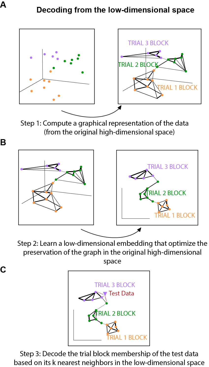
Here we give a very high level overview of the main steps of the decoding procedure (Fig. 5):
- Step 1- 2 is just the dimensionality reduction process. We have described Step 1 and 2 in part 1 of this post when introducing how UMAP works.
- Step 3 is the actual decoding step. Suppose that we are going to decode the trial identity of an example data point (purple triangle in Fig. 5C). We can simply use the k-nearest neighbor (KNN) algorithm to find the k nearest neighbors of the purple triangle, and then take the mode of the trial label of those nearest neighbors as the trial label for our purple triangle.
Part 4: Cross-validation with ‘leaving one trial out’
Now that we have a way to perform decoding, we need to properly quantify the decoding result with cross-validation.
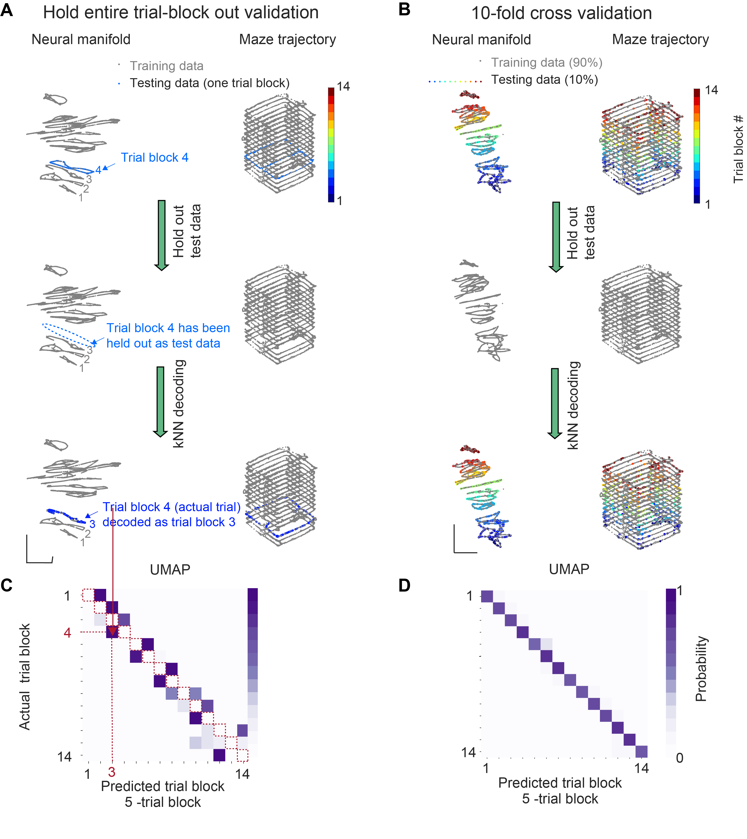
For cross-validation, we used the standard 10-fold cross-validation as well as the more targeted ‘leaving one trial out’ method. We want to highlight the ‘leaving one trial out’ cross-validation procedure here because we believe it is the most convincing evidence that the population activity pattern varied systematically across trials.
One important property of decoding is that as long as the different activity patterns of different trials are sufficiently differentiable, they can be decoded – they don’t have to be structured to be decodable.What we want to demonstrate here is that not only the population activity between different events are different (and thus decodable), they are also highly structured. Thus. we need to find a method from which we can conclude not only decodability, but also demonstrate structured variation across trials!
‘Leaving one trial out’ is such a method (Fig. 6). To elaborate, ‘leaving one trial out’ is expected to yield high decoding accuracy only if the state space of the data changed in a structured way, evolving along one axis according to the sequence of trial events. This is because this validation method makes sure that the training set does not contain any data that shar the trial block membership with the test set, the test data could be decoded only to the next closest trial block (but not the same trial block) in the state space (Fi6. 5C). Note that this is why the diagonal (red dashed line) of the confusion matrix had 0 decoding probability – the training and test data did not share any data from the same trial block and so cannot be decoded to the same trial block. If the neural embedding is structured according to the progression of trial events in time, the test data will be correctly decoded to their nearest neighbors and occupy the space immediately next to the diagonal of the confusion matrix.
Click here to read the full figure legend.
(A) Illustration of the hold entire trial block out validation method. Top, neural manifold from all the data in one example session. To give an example of the cross-validation procedure, data from one trial block (trial block 4; blue) was highlighted. Middle, the highlighted trial block in A was held out as test data. After removing the test data, a kNN decoder was trained only using training data (grey). Bottom, the test data was then embedded with the learned manifold (generated from training data), and the kNN decoder was used for trial block membership decoding. Test data was decoded to the trial block label of its nearest neighbor (trial block 3) on the training data manifold. Training data was gray and test data was colored by the identity of the decoded trial block.
(B) Illustration of the 10-fold cross-validation method. Top, neural manifold generated from all the data in one example session. 10% of the data were highlighted (colored by their true trial block identity). The highlighted data was held out as test data. Middle, after removing the t est data, a kNN decoder was trained only using training data (grey). Bottom, embedding the test data with the training manifold and us ing the kNN decoder for trial block identity decoding. Training data was gray and test data was colored by the identity of the decoded trial block (trial block 3).
(C) Confusion matrix obtained using hold entire trial block out validation. Note that the diagonal (red dashed line) of the confusion matrix had 0 decoding probability because the training and test data did not share any data from the same trial block. Since the neural embedding was structured according to the progression of trial events, the test data were correctly decoded to their nearest neighbors.
(D) Confusion matrix from UMAP trial block decoding using hold entire trial block out validation.
Part 5: Decoding from the original high-dimensional space and PCA space
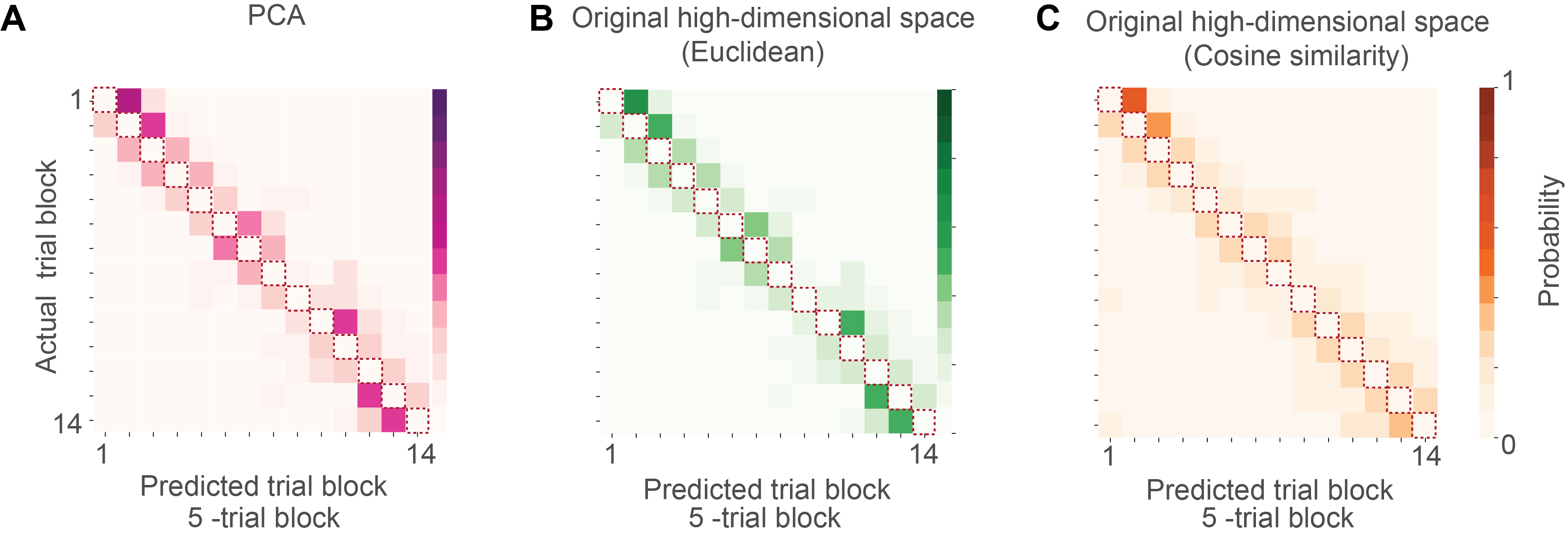
Can we trust the decoding result from the UMAP embedding? We know that dimensionality reduction can potentially distort the relationship between data points in the original dimensional space. In order to make sure our conclusion is not the result of potential distortion during the UMAP dimensionality reduction process, we decoded from the original high-dimensional space (Fig.6 B and C) as well as PCA space (Fig.7 A).
We can decode from the PCA space in an analogous way as decoding from the low dimensional embedding from UMAP. Our previous post showed that PCA does not generate good visualization comparing to UMAP (Fig. 7 A and B). However, that does not mean that we cannot decode from the PCA space! As we increase the number of principal components in the low-dimensional space, we can see that the decoding error actually decrease (Fig.7 D). If we use the first 15 principal components (decoding from a 15 dimensional space), the decoding accuracy is already comparable with decoding from the UMAP space (Fig.7 C and E).
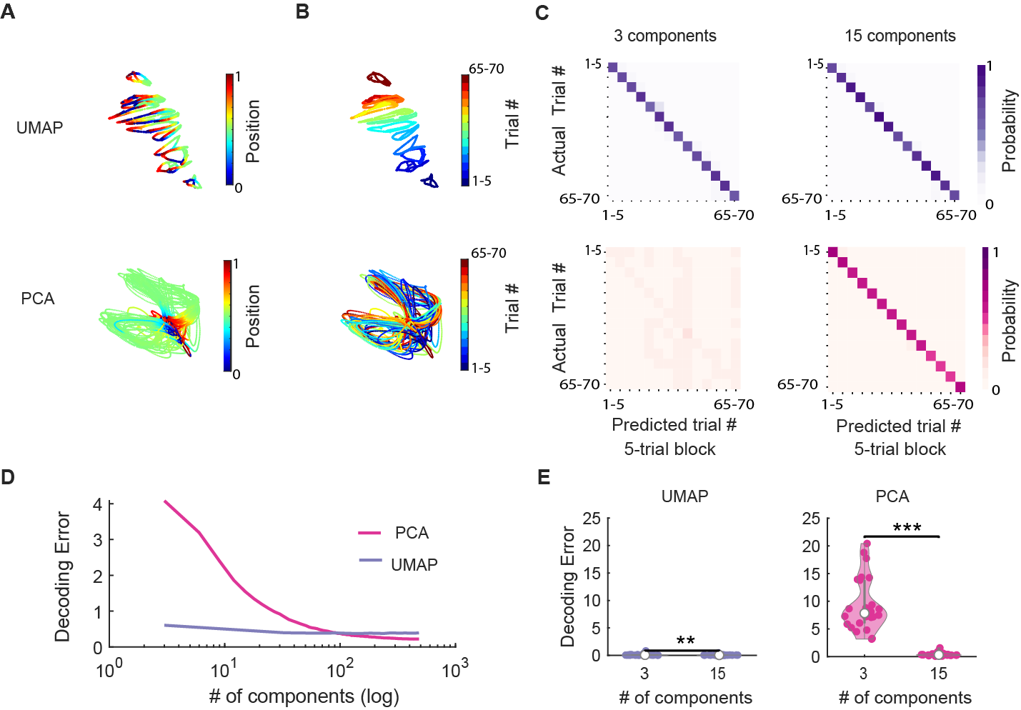
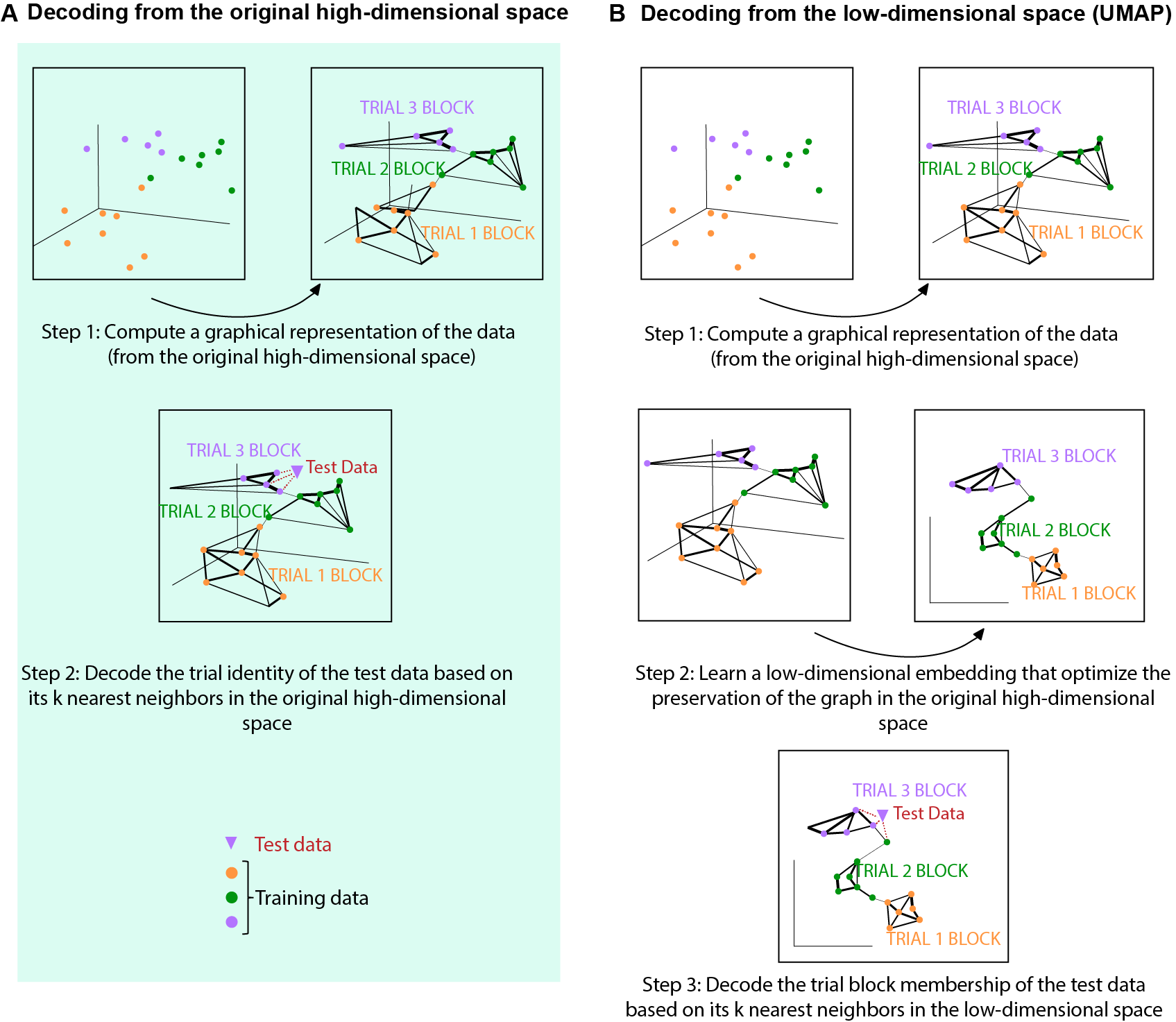
Fig. 8A illustrates the main steps of decoding from the original high dimensional space. As you can see, it follows the similar basic logic as decoding from the low-dimensional space (Fig.8 B). The only difference is that instead of performing kNN on the low-dimensional space, kNN was applied on the original high-dimensional space.
Another point worth to note when decoding from the high dimensional space is that when finding the nearest neighbour for decoding, the notion of distance is inevitable. What is the correct distance metric to use? In our paper, we compared both Euclidean distance, as well as the cosine similarity as distance metric.
Click here to read the full figure legend.
(A) Diagram explaining the main steps of trial block decoding from the original high -dimensional space. Step 1: by default, a weighted nearest neighbor (kNN) graph, which connects each datapoint to its nearest neighbors, was constructed and used to generate the initial topological representation of the training dataset (dots in three different colors). Step 2: the trial block membership of the test data (purple triangle) was decoded by taking the mode of its k nearest neighbors. For example, the example test data point (purple triangle) was decoded to be trial block 3 because all of its three nearest neighbors in the original high-dimensional space belong to trial block 3 (purple).
(B) Diagram explaining the main steps of trial block decoding from the low -dimensional space generated by UMAP. Step 1 was the same as in panel (A). Step 2: optimize the low -dimensional representation to preserve the topological representation as much as possible to that in the original high-dimensional space. Step 3: The trial block membership of the test data (purple triangle) was decoded by taking the mode of its nearest neighbors in the low -dimensional embedding. For example, the example test data point (purple triangle) was decoded to be trial block 3 because all its three nearest neighbors in the low -dimensional space belong to trial 3 block (purple).
As we can see, all those methods yield consistent conclusion with UMAP (Fig 9).
Part 6: Can we use UMAP for trial decoding?
UMAP can potentially introduce distortion during the dimensionality reduction process, and those distortions could affect the accuracy of the trial decoding results. In oder to demonstrate that we could use UMAP for trial decoding, we need to demonstrate that the trial block membership is consistent between the high and low-dimensional space.
Recall that we search for the k nearest neighbor of the test data and use their trial label as the trial label for the test data. This procedure can be applied to both the high-dimensional space as well the low-dimensional space. In order to test if UMAP introduce any distortion for trial membership decoding, for each data point, we can simply compute the consistency of the trial membership of the k nearest neighbours in the high-dimensional space and the low-dimensional UMAP embedding! If the trial membership the neighbours are consistent, then this means the UMAP dimensionality reduction process does not introduce distortion that affect accuracy of the trial membership decoding.
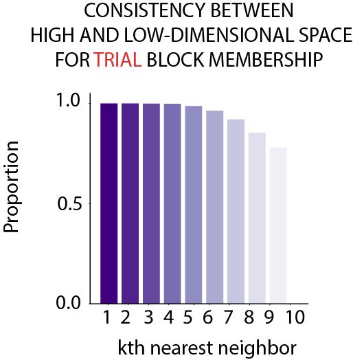
As we can see from Fig.10, the trial membership of the first 4 nearest neighbours between the high and low-dimensional space is 100% consistent! Note that this is not to say that UMAP perfectly preserve every little detail in the original high-dimensional space, rather this is to say that potential distortion that occurs at the dimensionality reduction process does not affect the trial decoding membership. Thus, we can use UMAP to quantify trial decoding.
Click here to read the full figure legend.
To check whether the UMAP dimensionality reduction process introduced distortions that affected the decoded trial block membership (5-trial block), the consistency between the original high- dimensional space and reduced low- dimensional space was plotted. For each data point, the decoded trial block membership of its ten nea rest neighbors in the high-dimensional space and the reduced low-dimensional space were compared. A data point was considered as having consistent trial block membership if trial_high - trial_low = 0 (i.e. being decoded to the same trial block). For the first four nearest neighbors , the decoded trial block membership between the high and low-dimensional space was 100% consistent. Thus, UMAP dimensionality reduction did not introduce any distortion at the level of trial block decoding results.
Part 7: Can electrode drift explain what we see?
Another important issue we need to properly address is recording stability. We need to exclude the possibility that the representation drift is not an artifact of electrode drift.
To this end, we plotted the amplitude of waveform over time as well as compared the spike amplitude in the first quarter and the last quarter of the session (Fig. 11). In addition, we also quantified waveform centroid displacement across time following Schoonover et al..
We also did additional comprehensive analysis to demonstrate that excluding the most unstable units does not change our conclusion. For readers interested in this, you can refer to our paper (Fig. S9) for more details.
Our analyses indicate that electrode drift cannot explain the representational drift.
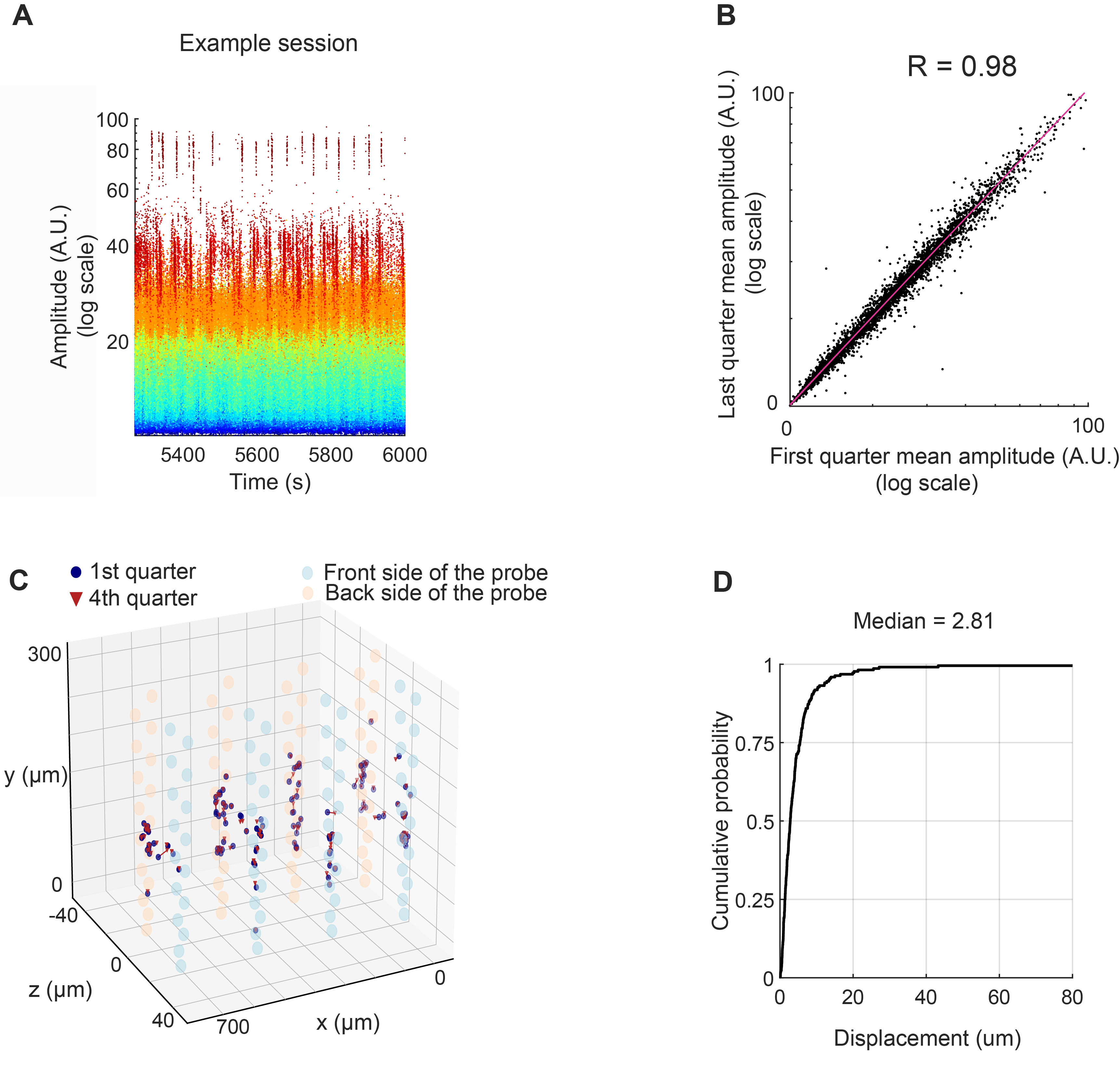
Click here to read the full figure legend.
(A) Waveform amplitude over time (on-maze duration) for all the cells in an example session. Spikes of individual neurons are color-coded by amplitude. The spike amplitude value was extracted from Amplitudes.npy, which was generated by Kilosort/Phy. It is a measure of each spike’s amplitude in the template space.
(B) Scatter plot of waveform amplitude in the first quarter of on- maze recording compared to the last quarter , for all the isolated units from the entire figure-8 maze dataset (Pearson correlation coefficient, N = 4469 cells from 6 animals).
(C) Single-unit waveform centroid displacement across time, from a representative session , plotted in 3-D space. Centroid was computed by taking the spatial average across electrode positions weighted by the squared mean waveform amplitude at each electrode (see Methods for details). Waveform centroid for each single unit during the first quarter (blue circles) and last quarter of recording (red triangles) were connected by red lines (note: most of them were very short and not visible). The large semi-transparent orange and blue circles indicate the positions of the dual-sided probe’s 128 electrode sites (blue, and orange, front and back sides of the dual-sided probe, respectively).
(D) Cumulative distribution of unit centroid displacement between the first and the last quarter of maze recording for all the cells in the dataset (median = 2.81- um, Q1 = 1.37- um, Q3 = 5.46- um; N= 4469 cells from 6 animals).
How to cite us ?
Enjoyed reading this post and found our demo code useful? It can be cited as follows:
Wannan Yang, Chen Sun, Roman Huszár, Thomas Hainmueller, Kirill Kiselev, György Buzsáki. “Selection of experience for memory by hippocampal sharp wave ripple.” Science 383, 1478-1483 (2024).

You can access the paper from the Science website here , the project website here, or from the Buzsaki lab website here.