The companion notebook will walk you through the steps of visualizing data with UMAP!

🔗 Follow the demo code in Colab Notebook here ! You will learn how we generated the UMAP visualization from raw spiking data!

NOTE!

Figures (black background) in this page are mostly interactive plots, and they might take a few seconds to load! You can rotate, zoom in and play with the manifold.

Part 1: Motivation

Using dual-side silicon probe, we were able to record from many hundreds of neurons simultaneously in the dorsal CA1 region of the hippocampus while the animal perform the figure-8 maze task. Animals were trained to alternative between left and right side of the arm to gain reward (located at the top left and top right corner of the maze (Fig. 1). The running trajectory of one example session was plotted (Fig.1, left). The trajectory was colored by the linearized position of the animal on the maze. The part of the maze in blue is where the trial start, the green areas on both sides of the maze are where the animal get rewarded, and the red parts of the maze are the end of the trial where animals return to the starting area and wait for the next trial to start.

In this example session, animal run for 70 trials, the trial by trial running trajectory was plotted and colored by trial number (fig. 1, right).

Fig 1. (Left) The illustration of the Figure-8 maze task, where mice alternated between left and right arms for water reward (blue droplets). The animal’s trajectory along maze corridors was color-coded by its linearized position. (Right) The running trajectories of a mouse running on the figure 8 maze, colored by trial block number.

When we inspected single neuron activity, we found that many neurons changed their firing rates across trials. Some cells fired with higher firing rates during early trials, some fired with higher firing rate during late trials, and some cells’ place field remapped across trials. The behavior of those individual cells gave us a hint that we might be able to distinguish which trial the animal is currently at based on the different spiking patterns of the CA1 neurons across trials. Since single cell activity is noisy, we wondered if we can find a way to leverage the activity of many hundreds of cells. And if so, we might be able to accurately decode which trial the animal is currently at based on population activity rather than activities of single cells.

Fig 2. Spatial tuning curve of example cells.

Click here to read the full figure legend.

The firing rate in space (linearized position on the figure-8 maze) of 3 example neurons across different trials in one representative session. The tuning curves were color-coded by trial block number (cold color for early trials and warm color for late trials). For each example cell, its firing rates as a function of the linearized position (from 0 to 200-cm) were plotted.

(A) An example cell that fired with higher firing rates during early trials.

(B) An example cell that fired with higher firing rate during late trials.

Part 2: Dimensionality Reduction

Humans are visual creatures. Good visualization can give us valuable intuition of the structure of the data that is otherwise hard to grasp.

The dual sided probe we used for recording allows us to record up to 500 neurons simultaneously. But the large number of neurons in our data means we are dealing with high dimensional data (the number of dimension scales with the number of neurons). When we have one neuron, visualizing the activity of that single cell across time is easy – the tuning curve in the fig. 2 above can give us a clear picture of how individual cell activity evolve across positions and across trials. But as soon as we have more than three neurons, we lost our ability to visualize the dynamics of the population activity in one coherent picture.

That is where dimensionality reduction becomes handy. Dimensionality reduction is a technique used to reduce the number of features in a dataset while retaining as much of the important information as possible. In other words, it is a process of transforming high-dimensional data into a lower-dimensional space that still preserves the essence of the original data (Although some aspects of the data will be distorted during the process of course, for more discussions on this, check out our next demo).

We used Uniform Manifold Approximation and Projection (UMAP) to embed the data in a low-dimensional space. The following interactive plots were generated by running UMAP on neural data recorded from the dorsal CA1 of the hippocampus when mouse performing an alternation task on the figure-8 maze. You can play with the visualization by dragging the interactive plot and rotate it to different angles.

Fig 3. An interactive plot showing the UMAP embedding of the neural data when a mouse was running on the figure-8 maze. (Left) UMAP embedding of population activity. Each point corresponds to the low-dimensional representation of one binned spiking data. (Right) running trajectory of a mouse on the figure-8 maze. Both the neural manifold and the running trajectory were colored by the animal's linearized position.

TIP!

This is an interactive plot! You can rotate the manifold and examine the manifold from different angles!! This figure might take a few seconds to render!

Fig 4. Similar to the previous plot, this interactive plot shows the UMAP embedding of the neural data when a mouse was running on the figure-8 maze.Both the neural manifold and the running trajectory were colored by trial block number.

As expected, UMAP visualization revealed that population activity of the hippocampus corresponded to a latent space that topologically resembled the physical environment. This visualization was beautiful yet not surprising since we know that there are place cells in the hippocampus.

What was really surprising and unexpected was when we colored the neural manifold with trial number, we saw a prominent progression of states that corresponded to trial sequences. This means that population activity in the hippocampus indeed encode the sequence of different events!

Heraclitus once said that “No man ever steps in the same river twice. For it’s not the same river and he’s not the same man.” Well, the brain is also not the same brain! Even though the animal visited the same places many times repeatedly, the neural activity was never the same again! It changes each time ⏳. Moreover, it changes in a very systematic way, organized in the same order as the unfolding of the events in time!

Part 3: UMAP visualization on different datasets

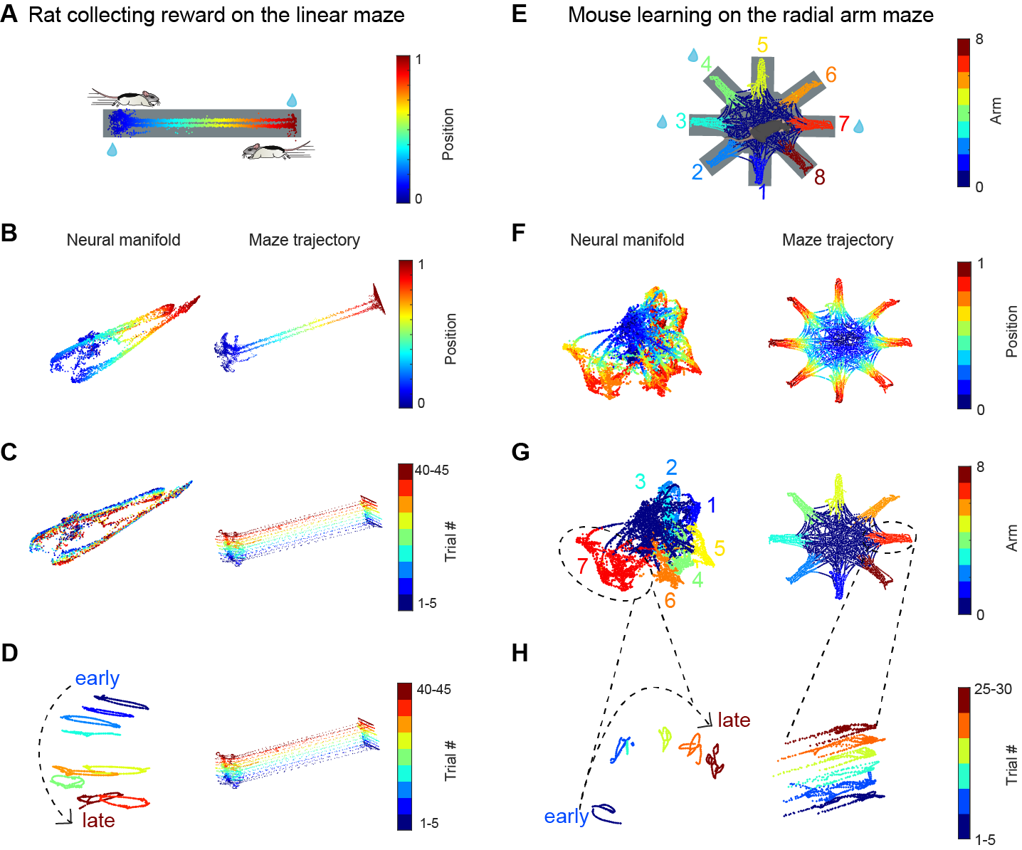
Trial specific population activity dynamics was also observed in simpler tasks like a linear maze, as well as more complex tasks like radial arm maze. Those observations suggest that the phenomenon we found is a general representation scheme used by the brain, regardless of behavioral paradigm and rodent species.

fig 5. Trial-specific evolution of neuronal population activity can be observed in different tasks and rodent species.

Click here to read the figure legend

(A) Rat running back and forth between the two reward ports located at either end of the linear track to collect water reward (blue droplets).

(B) Animal’s trajectory along the track was color-coded by animals’ linearized position along the track. Only data when the animal’s speed was larger than 1 cm/s was included. Left, UMAP embedding of population activity, colored by the rat’s linearized position. Right, running trajectory of a rat on the linear maze.

(D) Same session as (B) and (C), but using semi-supervised UMAP trained on blocks of 5 trials. The neural manifold (left) and maze trajectory (right) were colored by trial block number.

(E) In the radial-arm maze experiment, mouse collect water reward (blue droplets) from 3 out of the 8 potential reward sites at the end of each arm of the radial arm maze (arms 3,4 and 7 were rewarded in this example session). The animal’s trajectory along the track was color-coded by the arm’s identity.

(F) Left, UMAP embedding of population activity, colored by animal’s linearized position on each of the 8 arms. Right, running trajectory of a mouse on the radial arm maze.

(G) Same session as (F) but the neural manifold and maze trajectory were colored by arm identity. 0 represents the center area.(H) Since the manifold of figure-8 maze was complex, we focused only on one of the 8 arms to have a clear visualization of the state space evolution with trial number. We focused on arm 7 because the mouse visited this arm for 30 trials on this recording day. The neural manifold (left) was trained using semi-supervised UMAP on blocks of 5 trials. The manifold (left) and maze trajectory (right) were colored by trial block number.

Part 4: Why UMAP?

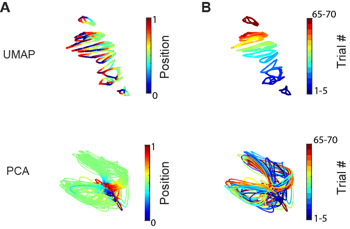
At this point, you might be wondering why we use UMAP and not simple linear dimensionality reduction methods like PCA. The short answer is that PCA does not generate as great visualization in the low dimensional space (3D). However, PCA can still be used for decoding if including more principal component (working in a higher dimensional space). Check out our next demo for further discussion regarding different methods!

Fig 7. Comparing UMAP and PCA. (A) Low- dimensional embedding of CA1 population activity, colored by animal’s linearized position on the figure-8 maze. Top, UMAP manifold. Bottom, PCA manifold. (B) Same as (A) but colored by trial block number. embedding.

Part 5: Down-sampling and its impact on neural embedding

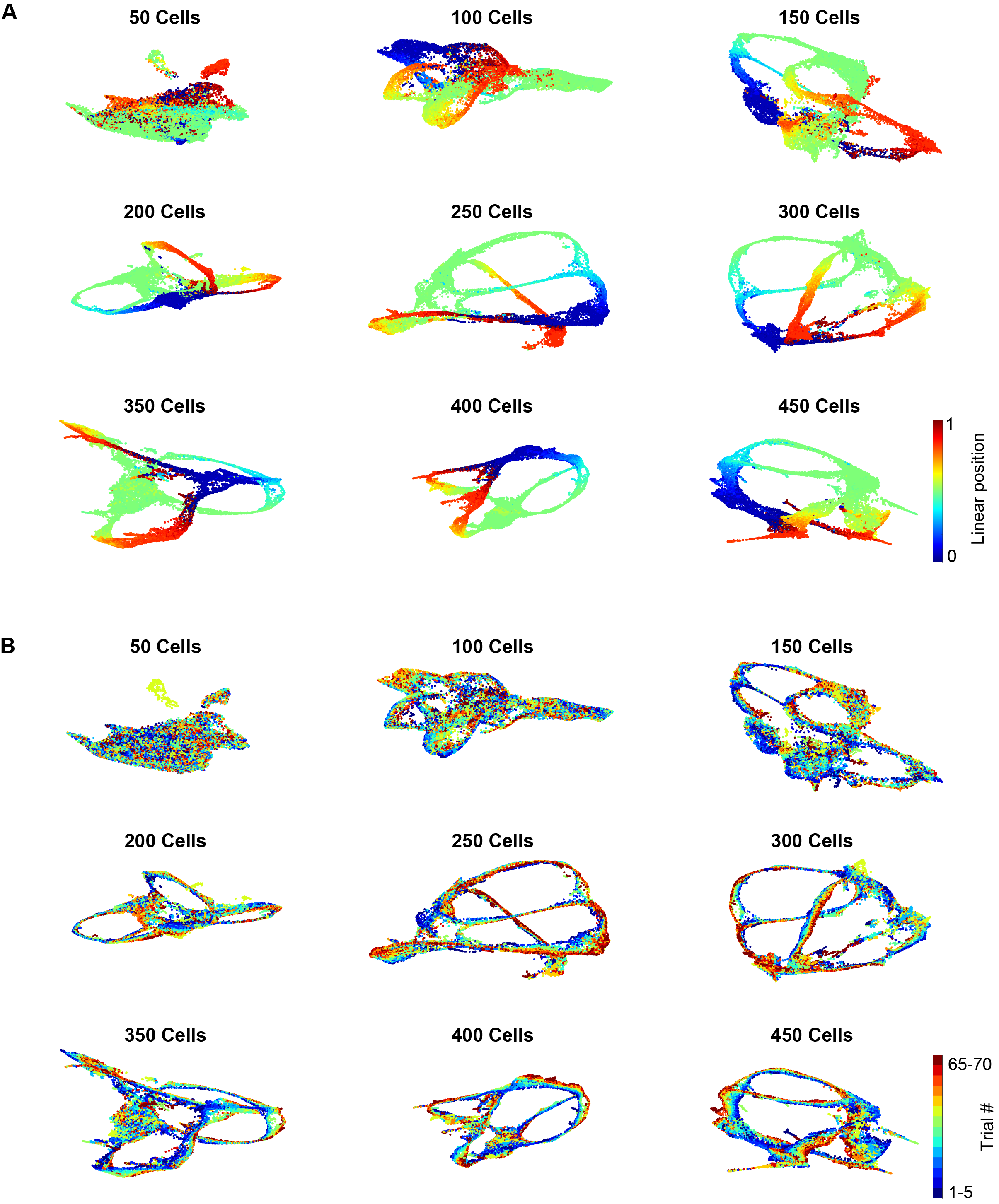
When we down-sampled the number of cells included for generating the UMAP embedding, we observed that the trial specific pattern degraded. When there were less than 100 cells, different trials were almost indistinguishable. This simple down-sampling analysis shows the importance of recording from large population of cells (thanks to the dual-sided probe that maximize the number of simultaneously recorded cells)!

Fig 6. Manifolds generated from down-sampling the number of cells included for UMAP embedding.

How to cite us ?

Enjoyed reading this post and found our demo code useful? Our paper can be cited as follows:

Wannan Yang, Chen Sun, Roman Huszár, Thomas Hainmueller, Kirill Kiselev, György Buzsáki. “Selection of experience for memory by hippocampal sharp wave ripple.” Science 383, 1478-1483 (2024).

You can access the paper from the Science website here , the project website here, or from the Buzsaki lab website here.